Deep learning Project : Stock price Analysis

Stock Price Analysis with LSTM

General Information about RNN models

• In the last few years, there have been incredible success applying RNNs to a variety of problems: speech recognition, language modeling, translation, image captioning.
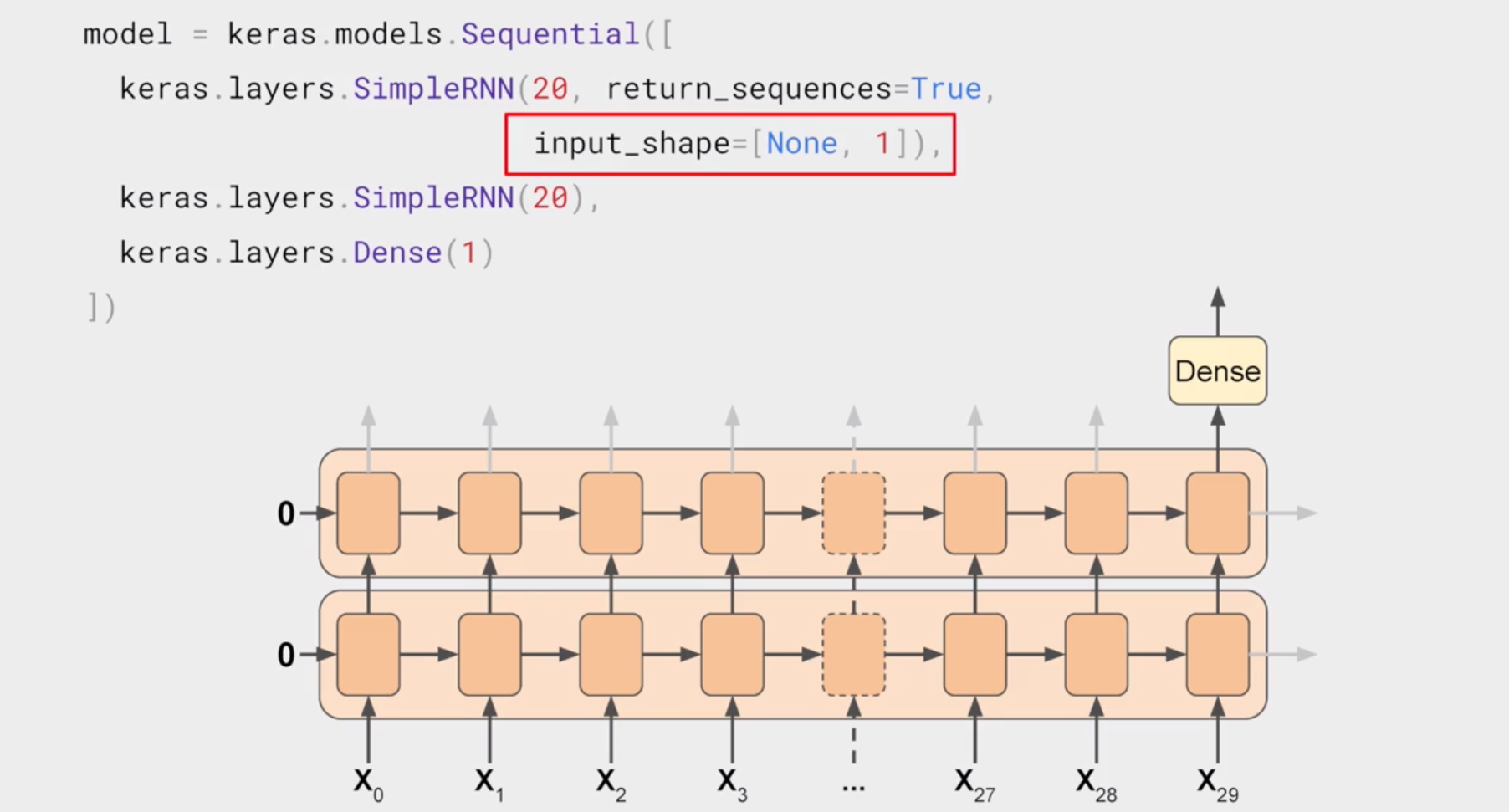
• RNN and LSTM and derivatives use mainly sequential processing over time. See the horizontal arrow in the diagram below:
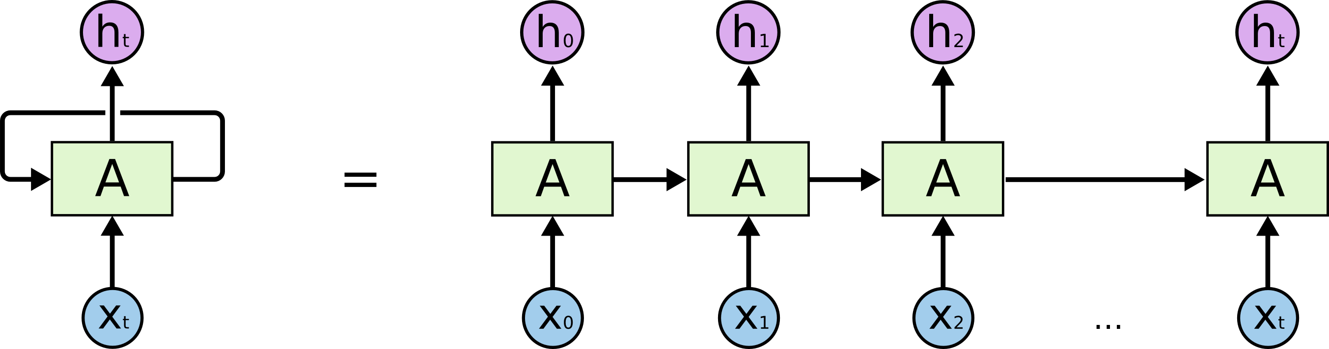
• This arrow means that long-term information has to sequentially travel through all cells before getting to the present processing cell. This means it can be easily corrupted by being multiplied many time by small numbers < 0. This is the cause of vanishing gradients.
• To the rescue, came the LSTM module, which today can be seen as multiple switch gates, and a bit like ResNet it can bypass units and thus remember for longer time steps. LSTM thus have a way to remove some of the vanishing gradients problems

  Architecture of LSTMs

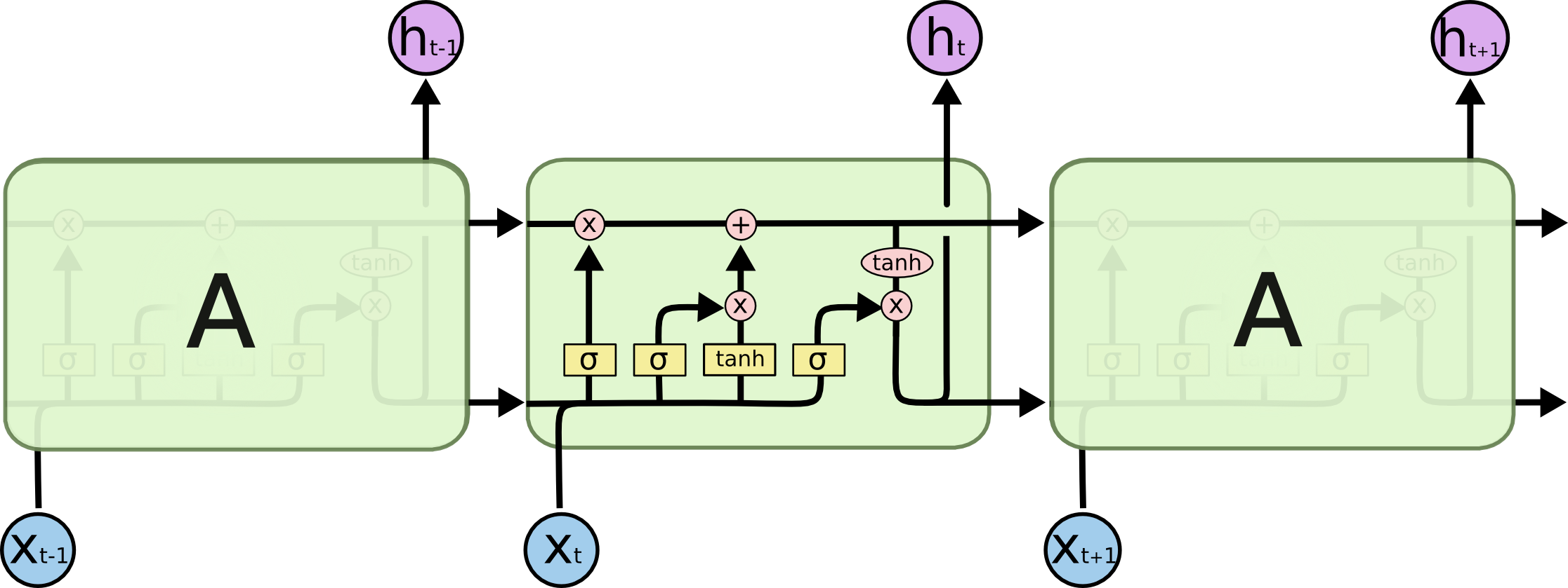
• A typical LSTM network is comprised of different memory blocks called cells (the rectangles that we see in the image). There are two states that are being transferred to the next cell; the cell state and the hidden state. The memory blocks are responsible for remembering things and manipulations to this memory is done through three major mechanisms, called gates. Each of them is being discussed below.
• 1. Forget gate:
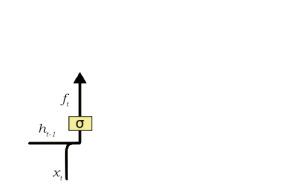
• A forget gate is responsible for removing information from the cell state. The information that is no longer required for the LSTM to understand things or the information that is of less importance is removed via multiplication of a filter. This is required for optimizing the performance of the LSTM network.
• This gate takes in two inputs; h_t-1 and x_t.
  • h_t-1 is the hidden state from the previous cell or the output of the *previous cell
  • x_t is the input at that particular time step
• 2. Input Gate
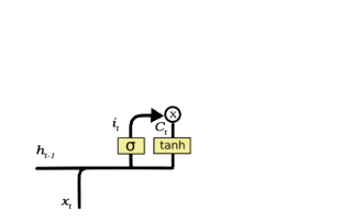
• The input gate is responsible for the addition of information to the cell state. This addition of information is basically three-step process as seen from the diagram above.
  • Regulating what values need to be added to the cell state by involving a sigmoid function. This is basically very similar to the forget gate and acts as a filter for all the information from h_t-1 and x_t.
  • Creating a vector containing all possible values that can be added (as perceived from h_t-1 and x_t) to the cell state. This is done using the tanh function, which outputs values from -1 to +1.
  • Multiplying the value of the regulatory filter (the sigmoid gate) to the created vector (the tanh function) and then adding this useful information to the cell state via addition operation.
• 3. Output Gate
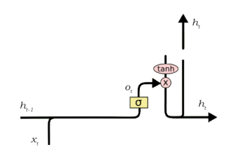
• The functioning of an output gate can again be broken down to three steps:
  • Creating a vector after applying tanh function to the cell state, thereby scaling the values to the range -1 to +1.
  • Making a filter using the values of h_t-1 and x_t, such that it can regulate the values that need to be output from the vector created above. This filter again employs a sigmoid function.
  • Multiplying the value of this regulatory filter to the vector created in step 1, and sending it out as a output and also to the hidden state of the next cell.

My model to estimate the next close value of this particular Stock

• Import the data which include 10 years of the particular stock history and then separate the data as train and test
  • Train ==> until 2019 (10 years of history)
  • Test ==> from Jan 2019 to March 2019 (unseen data to eval the model performance)
• Preprocess the data for input of the model. Basically, created a input including 60 days series data
• Visualize the data over time
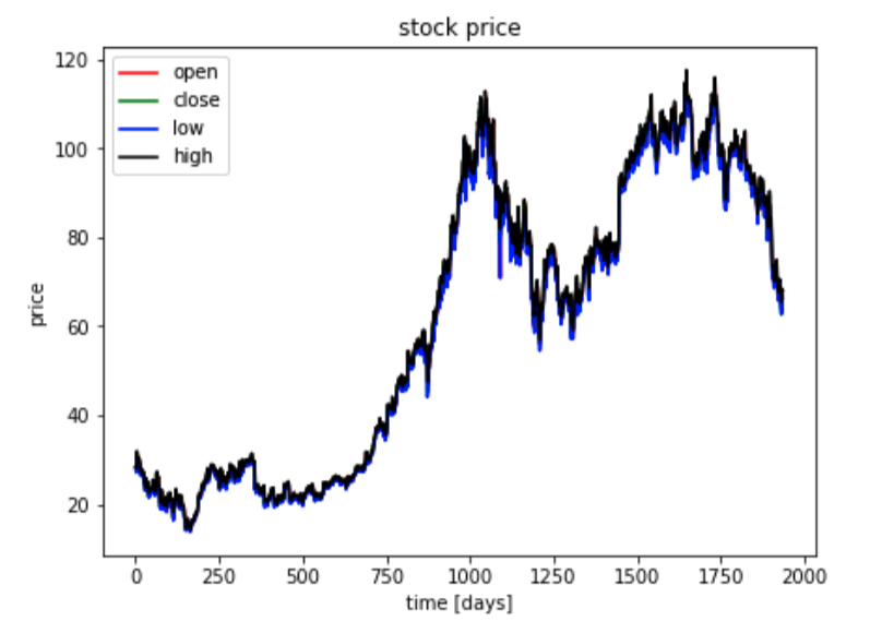
• Checked the correlation btw features and decide which feature will be used for this analysis
• Use past 60 days data to estimate the following date close value.
• Created a model with LSTM to remember long term history

from keras.layers import Input,Conv1D,TimeDistributed
from keras.models import Sequential
from keras.layers import Dense,TimeDistributed,Bidirectional
from keras.layers import LSTM,Input,Conv1D,TimeDistributed
from keras.layers import Dropout,Activation
from keras.callbacks import LearningRateScheduler
from keras.optimizers import SGD,Adagrad,Adam

model = Sequential([
    LSTM(60,return_sequences=True,input_shape =(None,1)),
    Dropout(0.6),
    Bidirectional(LSTM(60,return_sequences=True)),
    Dropout(0.6),
    Bidirectional(LSTM(60,return_sequences=True)),
    Dropout(0.6),
    Bidirectional(LSTM(30)),
    Dropout(0.4),
    Dense(60),
    Dropout(0.6),
    Dense(30),
    Dropout(0.35),
    Dense(1),
])

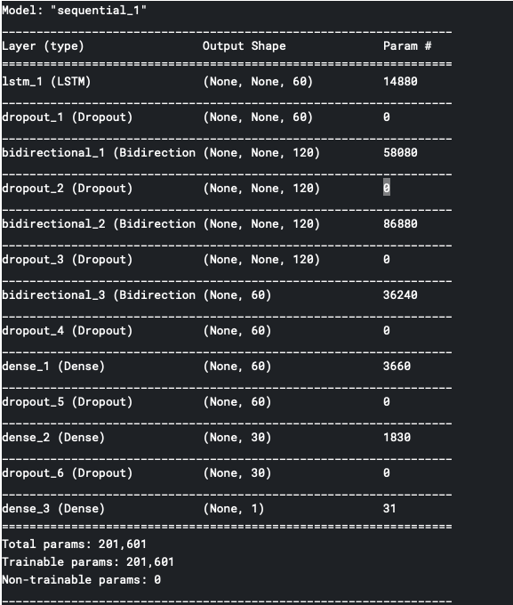
• Model summary :

• Train the model with learning rate scheduler so that I can capture the best learning rate in terms of time and accuracy
• Train the model with the learning rate we choose
• Test the model with unseen data and visualize the result against the real information

You might reach the repository through this link

Have fun!!!